
 E-mail Alert
 RSS
RSS
| Citation: |
Guo YM, Zhong LB, Min L, Wang JY, Wu Y et al. Adaptive optics based on machine learning: a review. Opto-Electron Adv 5, 200082 (2022). doi: 10.29026/oea.2022.200082

|
-
Abstract
Adaptive optics techniques have been developed over the past half century and routinely used in large ground-based telescopes for more than 30 years. Although this technique has already been used in various applications, the basic setup and methods have not changed over the past 40 years. In recent years, with the rapid development of artificial intelligence, adaptive optics will be boosted dramatically. In this paper, the recent advances on almost all aspects of adaptive optics based on machine learning are summarized. The state-of-the-art performance of intelligent adaptive optics are reviewed. The potential advantages and deficiencies of intelligent adaptive optics are also discussed.-
Keywords:
- adaptive optics /
- machine learning /
- deep learning
-

-
References
[1] Rao CH, Zhu L, Rao XJ, Zhang LQ, Bao H et al. Instrument description and performance evaluation of a high-order adaptive optics system for the 1m new vacuum solar telescope at Fuxian solar observatory. Astrophys J 833, 210 (2016). doi: 10.3847/1538-4357/833/2/210 [2] Kim D, Choi H, Brendel T et al. Advances in optical engineering for future telescopes. Opto-Electron Adv 4 (2021). doi: 10.29026/oea.2021.210040 [3] Tyson RK. Adaptive optics and ground-to-space laser communications. Appl Opt 35, 3640–3646 (1996). doi: 10.1364/AO.35.003640 [4] Kubby JA. Adaptive Optics for Biological Imaging (Taylor & Francis, Boca Raton, America, 2013). [5] Shi GH, Dai Y, Wang L, Ding ZH, Rao XJ et al. Adaptive optics optical coherence tomography for retina imaging. Chin Opt Lett 6, 424–425 (2008). doi: 10.3788/COL20080606.0424 [6] Booth MJ. Adaptive optical microscopy: the ongoing quest for a perfect image. Light Sci Appl 3, e165 (2014). doi: 10.1038/lsa.2014.46 [7] Bennet F, Thearle O, Roberts L, Smith J, Spollard SJ et al. Free-space quantum communication link with adaptive optics. (AMOS, 2018). [8] https://afresearchlab.com/news/afrl-demonstrates-worlds-first-daytime-free-space-quantum-communication-enabled-by-adaptive-optics/ [9] Burns SA, Elsner AE, Sapoznik KA, Warner RL, Gast TJ. Adaptive optics imaging of the human retina. Prog Retin Eye Res 68, 1–30 (2019). doi: 10.1016/j.preteyeres.2018.08.002 [10] Jiang WH. Overview of adaptive optics development. Opto-Electron Eng 45, 170489 (2018). doi: 10.12086/oee.2018.170489 [11] Rao CH, Zhu L, Zhang LQ et al. Development of solar adaptive optics. Opto-Electron Eng 45, 170733 (2018). doi: 10.12086/oee.2018.170733 [12] Wei K, Zhang XJ, Xian H, Ma WL, Zhang A et al. First light on the 127-element adaptive optical system for 1.8-m telescope. Chin Opt Lett 8, 1019–1021 (2010). doi: 10.3788/COL20100811.1019 [13] Yang ZP, Li ED, Zhang XJ, Fan MW, Shi NP et al. Adaptive optics correction systems on Shen Guang III facility. Opto-Electron Eng 45, 180049 (2018). [14] Liu C, Chen SQ, Li XY, Xian H. Performance evaluation of adaptive optics for atmospheric coherent laser communications. Opt Express 22, 15554–15563 (2014). doi: 10.1364/OE.22.015554 [15] Zhao JL, Xiao F, Kang J, Zhao HX, Dai Y et al. Quantifying intraocular scatter with near diffraction-limited double-pass point spread function. Biomed Opt Express 7, 4595–4604 (2016). doi: 10.1364/BOE.7.004595 [16] Guo YM, Zhang A, Fan XL, Rao CH, Wei L et al. First on-sky demonstration of the piezoelectric adaptive secondary mirror. Opt Lett 41, 5712–5715 (2016). doi: 10.1364/OL.41.005712 [17] Rao CH, Zhang LQ, Kong L, Guo YM, Rao XJ et al. First light of solar multi-conjugate adaptive optics at the 1-m new vacuum solar telescope. Sci China Phys, Mech Astron 61, 089621 (2018). doi: 10.1007/s11433-017-9178-6 [18] Rao CH, Gu NT, Rao XJ, Li C, Zhang LQ et al. First light of the 1.8-m solar telescope–CLST. Sci China Phys, Mech Astron 63, 109631 (2020). doi: 10.1007/s11433-019-1557-3 [19] Chen M, Liu C, Rui DM, Xian H. Experimental results of 5-Gbps free-space coherent optical communications with adaptive optics. Opt Commun 418, 115–119 (2018). doi: 10.1016/j.optcom.2018.03.003 [20] Guan CL, Zhang XJ, Deng JM et al. Deformable mirror technologies at Institute of Optics and Electronics, Chinese Academy of Sciences. Opto-Electron Eng 47, 200337 (2020). doi: 10.12086/oee.2020.200337 [21] Huang LH, Rao CH. Wavefront sensorless adaptive optics: a general model-based approach. Opt Express 19, 317–379 (2011). doi: 10.1364/OE.19.000317 [22] Assémat F, Gendron E, Hammer F. The FALCON concept: multi-object adaptive optics and atmospheric tomography for integral field spectroscopy – principles and performance on an 8-m telescope. Mon Not Roy Astron Soc 376, 287–312 (2007). doi: 10.1111/j.1365-2966.2007.11422.x [23] Macintosh B, Troy M, Doyon R, Graham J, Baker K et al. Extreme adaptive optics for the Thirty Meter Telescope. Proc SPIE 6272, 62720N (2006). doi: 10.1117/12.672032 [24] LeCun Y, Bengio Y, Hinton G. Deep learning. Nature 512, 436–444 (2015). [25] Angel JRP, Wizinowich P, Lloyd-Hart M, Sandler D. Adaptive optics for array telescopes using neural-network techniques. Nature 348, 221–224 (1990). doi: 10.1038/348221a0 [26] Sandler DG, Barrett TK, Palmer DA, Fugate FQ, Wild WJ. Use of a neural network to control an adaptive optics system for an astronomical telescope. Nature 351, 300–302 (1991). doi: 10.1038/351300a0 [27] Demailly L, Gendron E, Beuzit JL, Lacombe F, Hubin NN. Artificial Intelligence system and optimized modal control for the ADONIS adaptive optics instrument. Proc SPIE 2201, 867–878 (1994). doi: 10.1117/12.176120 [28] Wizinowich PL, Lloyd-Hart M, McLeod BA, Colucci D, Dekany RG et al. Neural network adaptive optics for the multiple-mirror telescope. Proc SPIE 1542, 148–158 (1991). doi: 10.1117/12.48802 [29] Lloyd-Hart M, Wizinowich P, McLeod B, Wittman D, Colucci D et al. First results of an on-line adaptive optics system with atmospheric wavefront sensing by an artificial neural network. Astrophys J 390, L41–L44 (1992). doi: 10.1086/186367 [30] Barrett TK, Sandler DG. Artificial neural network for the determination of Hubble Space Telescope aberration from stellar images. Appl Opt 32, 1720–1727 (1993). doi: 10.1364/AO.32.001720 [31] Montera DA, Welsh BM, Roggemann MC, Ruck DW. Prediction of wave-front sensor slope measurements with artificial neural networks. Appl Opt 36, 675–681 (1997). doi: 10.1364/AO.36.000675 [32] Davies R, Kasper M. Adaptive optics for astronomy. Ann Rev Astron Astrophys 50, 305–351 (2012). doi: 10.1146/annurev-astro-081811-125447 [33] Platt BC, Shack R. History and principles of Shack-Hartmann wavefront sensing. J Refract Surg 17, S573–S577 (2001). [34] Ragazzoni R. Pupil plane wavefront sensing with an oscillating prism. J Mod Opt 43, 289–293 (1996). doi: 10.1080/09500349608232742 [35] Roddier F. Curvature sensing and compensation: a new concept in adaptive optics. Appl Opt 27, 1223–1225 (1988). doi: 10.1364/AO.27.001223 [36] Noll RJ. Zernike polynomials and atmospheric turbulence. J Opt Soc Am 66, 207–211 (1976). doi: 10.1364/JOSA.66.000207 [37] Dai GM. Modal wave-front reconstruction with Zernike polynomials and Karhunen–Loève functions. J Opt Soc Am A 13, 1218–1225 (1996). doi: 10.1364/JOSAA.13.001218 [38] Boyer C, Michau V, Rousset G. Adaptive optics: Interaction matrix measurements and real time control algorithms for the COME-ON project. Proc SPIE 1271, 63–81 (1990). doi: 10.1117/12.20395 [39] Kulcsár C, Raynaud HF, Petit C, Conan JM, de Lesegno PV. Optimal control, observers and integrators in adaptive optics. Opt Express 14, 7464–7476 (2006). doi: 10.1364/OE.14.007464 [40] Petit C, Quiros-Pacheco F, Conan JM, Kulcsar C, Raynaud HF et al. Kalman-filter-based control for adaptive optics. Proc SPIE 5490, 1414–1425 (2004). doi: 10.1117/12.550775 [41] Petit C, Conan JM, Kulcsár C, Raynaud HF, Fusco T et al. First laboratory demonstration of closed-loop Kalman based optimal control for vibration filtering and simplified MCAO. Proc SPIE 6272, 62721T (2006). doi: 10.1117/12.671525 [42] Petit C, Conan JM, Kulcsár C, Raynaud HF, Fusco T. First laboratory validation of vibration filtering with LQG control law for Adaptive Optics. Opt Express 16, 87–97 (2008). doi: 10.1364/OE.16.000087 [43] Correia C, Conan JM, Kulcsár C, Raynaud HF, Petit C. Adapting optimal LQG methods to ELT-sized AO systems. In Proceedings of the 1st AO4ELT Conference 07003 (EDP Sciences, 2010); https://doi.org/10.1051/ao4elt/201007003. [44] Wang JY, Guo YM, Kong L, Rao CH. Experimental demonstration of LQG control with disturbance mitigation on multiple modes in adaptive optics system. Optik 202, 163594 (2020). doi: 10.1016/j.ijleo.2019.163594 [45] Wang JY, Guo YM, Kong L, Zhao LQ, Gu NT et al. Automatic disturbance identification for linear quadratic Gaussian control in adaptive optics. Mon Not Roy Astronom Soc 496, 5126–5138 (2020). doi: 10.1093/mnras/staa1698 [46] Doelman N, Osborn J. Modelling and prediction of non-stationary optical turbulence behavior. Proc SPIE 9909, 99091M (2016). doi: 10.1117/12.2233351 [47] Ayers GR, Dainty JC. Iterative blind deconvolution method and its applications. Opt Lett 13, 547–549 (1988). doi: 10.1364/OL.13.000547 [48] Ng MK, Plemmons RJ, Qiao SZ. Regularization of RIF blind image deconvolution. IEEE Trans Image Process 9, 1130–1134 (2000). doi: 10.1109/83.846254 [49] Thiébaut E, Conan JM. Strict a priori constraints for maximum-likelihood blind deconvolution. J Opt Soc Am A12, 485–492 (1995). [50] Paxman RG, Schulz TJ, Fienup JR. Joint estimation of object and aberrations by using phase diversity. J Opt Soc Am A 9, 1072–1085 (1992). doi: 10.1364/JOSAA.9.001072 [51] Löfdahl MG, Scharmer GB. Wavefront sensing and image restoration from focused and defocused solar images. Astron Astrophys Suppl Ser 107, 243–264 (1994). [52] Löfdahl MG, Berger TE, Shine RS, Title AM. Preparation of a dual wavelength sequence of high-resolution solar photospheric images using phase diversity. Astrophys J 495, 965–972 (1998). doi: 10.1086/305308 [53] Schulz TJ, Stribling BE, Miller JJ. Multiframe blind deconvolution with real data: imagery of the Hubble Space Telescope. Opt Express 11, 355–362 (1997). [54] Schulz TJ. Multiframe blind deconvolution of astronomical images. J Opt Soc Am A 10, 1064–1073 (1993). doi: 10.1364/JOSAA.10.001064 [55] Löfdahl MG. Multi-frame blind deconvolution with linear equality constraints. Proc SPIE 4792, 146–155 (2002). doi: 10.1117/12.451791 [56] Van Noort M, Van Der Voort R, Löfdahl MG. Solar image restoration by use of multi-frame blind de-convolution with multiple objects and phase diversity. Sol Phys 228, 191–215 (2005). doi: 10.1007/s11207-005-5782-z [57] Wöger F, van der Lühe O. Field dependent amplitude calibration of adaptive optics supported solar speckle imaging. Appl Opt 46, 8015–8026 (2007). doi: 10.1364/AO.46.008015 [58] Wöger F. Optical transfer functions derived from solar adaptive optics system data. Appl Opt 49, 1818–1825 (2010). doi: 10.1364/AO.49.001818 [59] Labeyrie A. Attainment of diffraction limited resolution in large telescopes by Fourier analysing speckle patterns in star images. Astron Astrophys 6, 85–87 (1970). [60] Weigelt GP. Modified astronomical speckle interferometry “speckle masking”. Opt Commun 21, 55–59 (1977). doi: 10.1016/0030-4018(77)90077-3 [61] Pehlemann E, van der Lühe O. Technical aspects of the speckle masking phase reconstruction algorithm. Astron Astrophys 216, 337–346 (1989). [62] Puschmann KG, Sailer M. Speckle reconstruction of photometric data observed with adaptive optics. Astron Astrophys 454, 1011–1019 (2006). doi: 10.1051/0004-6361:20053918 [63] Knox KT, Thompson BJ. Recovery of images from atmospherically degraded short-exposure photographs. Astron Astrophys 193, L45–L48 (1974). [64] van Noort M, van der Voort LR, Löfdahl MG. Solar image restoration by use of multi-object multi-frame blind deconvolution. In Solar MHD Theory and Observations: A High Spatial Resolution Perspective ASP Conference Series (ASP, 2006); https://ui.adsabs.harvard.edu/abs/2006ASPC..354...55V. [65] Puschmann KG, Beck C. Application of speckle and (multi-object) multi-frame blind deconvolution techniques on imaging and imaging spectropolarimetric data. Astron Astrophys 533, A21 (2011). doi: 10.1051/0004-6361/201116904 [66] Peck CL, Wöger F, Marino J. Influence of speckle image reconstruction on photometric precision for large solar telescopes. Astron Astrophys 607, A83 (2017). doi: 10.1051/0004-6361/201731275 [67] Zhong LB, Zhang LQ, Shi ZD, Tian Y, Guo YM et al. Wide field-of-view, high-resolution Solar observation in combination with ground layer adaptive optics and speckle imaging. Astron Astrophys 637, A99 (2020). doi: 10.1051/0004-6361/201935109 [68] Denker C, Yang G, Wang H. Near real-time image reconstruction. Solar Phys 202, 63–70 (2001). doi: 10.1023/A:1011886923189 [69] Wöger F, van der Lühe O. KISIP: a software package for speckle interferometry of adaptive optics corrected solar data. Proc SPIE 7019, 7019E (2008). doi: 10.1117/12.788062 [70] Guo T, Zhang B, Gu N T et al. Research on polarization Hartmann wavefront detection technology. Opto-Electron Eng 48, 210076 (2021). doi: 10.12086/oee.2021.210076 [71] Guo H, Korablinova N, Ren QS, Bille J. Wavefront reconstruction with artificial neural networks. Opt Express 14, 6456–6462 (2006). doi: 10.1364/OE.14.006456 [72] Swanson R, Lamb M, Correia C, Sivanandam S, Kutulakos K. Wavefront reconstruction and prediction with convolutional neural networks. Proc SPIE 10703, 107031F (2018). doi: 10.1117/12.2312590 [73] Li ZQ, Li XY. Centroid computation for Shack-Hartmann wavefront sensor in extreme situations based on artificial neural networks. Opt Express 26, 31675–31692 (2018). doi: 10.1364/OE.26.031675 [74] Gómez SLS, González-Gutiérrez C, Alonso ED, Rodríguez JDS, Rodríguez MLS et al. Improving adaptive optics reconstructions with a deep learning approach. In Proceedings of the 13th International Conference on Hybrid Artificial Intelligence Systems (Springer, 2018);https://doi.org/10.1007/978-3-319-92639-1_7. [75] DuBose TB, Gardner DF, Watnik AT. Intensity-enhanced deep network wavefront reconstruction in Shack–Hartmann sensors. Opt Lett 45, 1699–1702 (2020). doi: 10.1364/OL.389895 [76] Hu LJ, Hu SW, Gong W, Si K. Learning-based Shack-Hartmann wavefront sensor for high-order aberration detection. Opt Express 27, 33504–33517 (2019). doi: 10.1364/OE.27.033504 [77] Hu LJ, Hu SW, Gong W, Si K. Deep learning assisted Shack-Hartmann wavefront sensor for direct wavefront detection. Opt Lett 45, 3741–3744 (2020). doi: 10.1364/OL.395579 [78] Kendrick RL, Acton DS, Duncan AL. Phase-diversity wave-front sensor for imaging systems. Appl Opt 33, 6533–6546 (1994). doi: 10.1364/AO.33.006533 [79] Paine SW, Fienup JR. Machine learning for improved image-based wavefront sensing. Opt Lett 43, 1235–1238 (2018). doi: 10.1364/OL.43.001235 [80] Guo HY, Xu YJ, Li Q, Du SP, He D et al. Improved machine learning approach for wavefront sensing. Sensors 19, 3533 (2019). doi: 10.3390/s19163533 [81] Ma HM, Liu HQ, Qiao Y, Li XH, Zhang W. Numerical study of adaptive optics compensation based on Convolutional Neural Networks. Opt Commun 433, 283–289 (2019). doi: 10.1016/j.optcom.2018.10.036 [82] Wu Y, Guo YM, Bao H, Rao CH. Sub-millisecond phase retrieval for phase-diversity wavefront sensor. Sensors 20, 4877 (2020). doi: 10.3390/s20174877 [83] Nishizaki Y, Valdivia M, Horisaki R, Kitaguchi K, Saito M et al. Deep learning wavefront sensing. Opt Express 27, 240–251 (2019). doi: 10.1364/OE.27.000240 [84] Osborn J, Guzman D, de Cos Juez FJ, Basden AG, Morris TJ et al. Open-loop tomography with artificial neural networks on CANARY: on-sky results. Mon Not Roy Astron Soc 441, 2508–2514 (2014). doi: 10.1093/mnras/stu758 [85] Jorgenson MB, Aitken GJM. Prediction of atmospherically induced wave-front degradations. Opt Lett 17, 466–468 (1992). doi: 10.1364/OL.17.000466 [86] Lloyd-Hart M, McGuire P. Spatio-temporal prediction for adaptive optics wavefront reconstructors. In Proceedings of the European Southern Observatory Conference on Adaptive Optics (ESO, 1996);http://citeseerx.ist.psu.edu/viewdoc/download?doi=10.1.1.35.3278&rep=rep1&type=pdf. [87] van Kooten M, Doelman N, Kenworthy M. Impact of time-variant turbulence behavior on prediction for adaptive optics systems. J Opt Soc Am A 36, 731–740 (2019). doi: 10.1364/JOSAA.36.000731 [88] Doelman N, Fraanje R, Houtzager I, Verhaegen M. Adaptive and real-time optimal control for adaptive optics systems. Eur J Control 15, 480–488 (2009). doi: 10.3166/ejc.15.480-488 [89] Chen Y. LSTM recurrent neural network prediction algorithm based on Zernike modal coefficients. Optik 203, 163796 (2020). doi: 10.1016/j.ijleo.2019.163796 [90] Chen Y. Voltages prediction algorithm based on LSTM recurrent neural network. Optik 220, 164869 (2020). doi: 10.1016/j.ijleo.2020.164869 [91] Liu XW, Morris T, Saunter C, de Cos Juez FJ, González-Gutiérrez C et al. Wavefront prediction using artificial neural networks for open-loop adaptive optics. Mon Not Roy Astron Soc 496, 456–464 (2020). doi: 10.1093/mnras/staa1558 [92] Sun Z, Chen Y, Li XY, Qin XL, Wang HY. A Bayesian regularized artificial neural network for adaptive optics forecasting. Opt Commun 382, 519–527 (2017). doi: 10.1016/j.optcom.2016.08.035 [93] van Kooten M, Doelman N, Kenworthy M. Performance of AO predictive control in the presence of non-stationary turbulence. In Proceedings of the 5th AO4ELT Conference (Instituto de Astrofisica de Canarias, 2017); https://repository.tudelft.nl/view/tno/uuid%3A4a101b83-7e90-44f8-abaa-b7817cc8b16a. [94] Béchet C, Tallon M, Le Louarn M. Very low flux adaptive optics using spatial and temporal priors. In Proceedings of the 1st AO4ELT Conference 03010 (EDP Sciences, 2010); https://doi.org/10.1051/ao4elt/201003010 [95] Ramos AA, de la Cruz Rodríguez J, Yabar AP. Real-time, multiframe, blind deconvolution of solar images. Astron Astrophys 620, A73 (2018). doi: 10.1051/0004-6361/201833648 [96] Shi JL, Zhang RZ, Guo SP, Yang YK, Xu R et al. Space targets adaptive optics images blind restoration by convolutional neural network. Opt Eng 58, 093102 (2019). doi: 10.1117/1.OE.58.9.093102 [97] Ramos AA. Learning to do multiframe blind deconvolution unsupervisedly. arXiv: 2006.01438 (2020).https://doi.org/10.48550/arXiv.2006.01438 [98] Baso CJD, Ramos AA. Enhancing SDO/HMI images using deep learning. Astron Astrophys 614, A5 (2018). doi: 10.1051/0004-6361/201731344 [99] Zhou SC, Zhang JW, Pan JS, Zuo WM, Xie HZ et al. Spatio-temporal filter adaptive network for video deblurring. In Proceedings of 2019 IEEE/CVF International Conference on Computer Vision (IEEE, 2019);https://doi.org/10.1109/ICCV.2019.00257. [100] Xiao F, Zhao JL, Zhao HX, Yun D, Zhang YD. Deblurring adaptive optics retinal images using deep convolutional neural networks. Biomed Opt Express 8, 5675–5687 (2017). doi: 10.1364/BOE.8.005675 [101] Vorontsov MA, Sivokon VP. Stochastic parallel-gradient-descent technique for high-resolution wave-front phase-distortion correction. J Opt Soc Am A 15, 2745–2758 (1998). doi: 10.1364/JOSAA.15.002745 [102] Hu K, Xu B, Xu ZX, Wen LH, Yang P et al. Self-learning control for wavefront sensorless adaptive optics system through deep reinforcement learning. Optik 178, 785–793 (2019). doi: 10.1016/j.ijleo.2018.09.160 [103] Mnih V, Kavukcuoglu K, Silver D, Graves A, Antonoglou I et al. Playing Atari with deep reinforcement learning. arXiv: 1312.5602 (2013). https://doi.org/10.48550/arXiv.1312.5602. [104] Xu ZX, Yang P, Hu K, Xu B, Li HP. Deep learning control model for adaptive optics systems. Appl Opt 58, 1998–2009 (2019). doi: 10.1364/AO.58.001998 -
Access History

Figures(22)
Tables(7)
Article Metrics


Export File
Citation
Guo YM, Zhong LB, Min L, Wang JY, Wu Y et al. Adaptive optics based on machine learning: a review. Opto-Electron Adv 5, 200082 (2022). doi: 10.29026/oea.2022.200082
Format
Content
 DownLoad:


-
Figure 1.
Overview of AOS for solar observation. The light waves emitted by the Sun suffer from wavefront distortion when pass through the atmospheric turbulence. The WFS detects the intensity distributions caused by the wavefront distortion and then transfers them to the RTC. The RTC reconstructs the wavefront and calculates the voltages sent to the DM to compensate the distorted wavefront. Meanwhile, the scientific camera records the corrected images and sends them for post-processing in order to get even higher resolution.
-
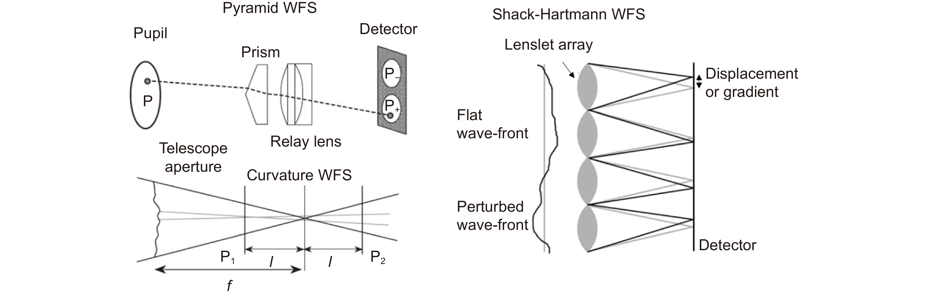
Figure 2.
Principles of three kinds of WFS. Figure reproduced with permisson from ref.32, Annual Reviews Inc.
-
Figure 3.
(a) The training algorithm of the ANN where displacements of the spots are taken as the inputs while the Zernike coefficients as outputs. To make the network more insensitive to the noise in the spot patterns, the training is also performed on noisy patterns. The noise added to the spot displacements follows Gaussian distribution. (b) The average reconstructed errors of ANNs with different number of neurons in the hidden layer shows that hidden layer with 90 neurons performs best. (c) Comparison of residual errors of LSF, SVD and ANN algorithms. Figure reproduced from ref.71, Optical Society of America.
-
Figure 4.
(a) The classification network similar to CoG method for spot detection with 50 hidden layer neurons named as SHNN-50. (b) The classification network with 900 hidden layer neurons named as SHNN-900. The input is the flattened subaperture image (25×25) and the output is a kind of classification in 625 classes, the same as the number of pixels indicating the potential center of the spot. Figure reproduced from ref.73, Optical Society of America.
-
Figure 5.
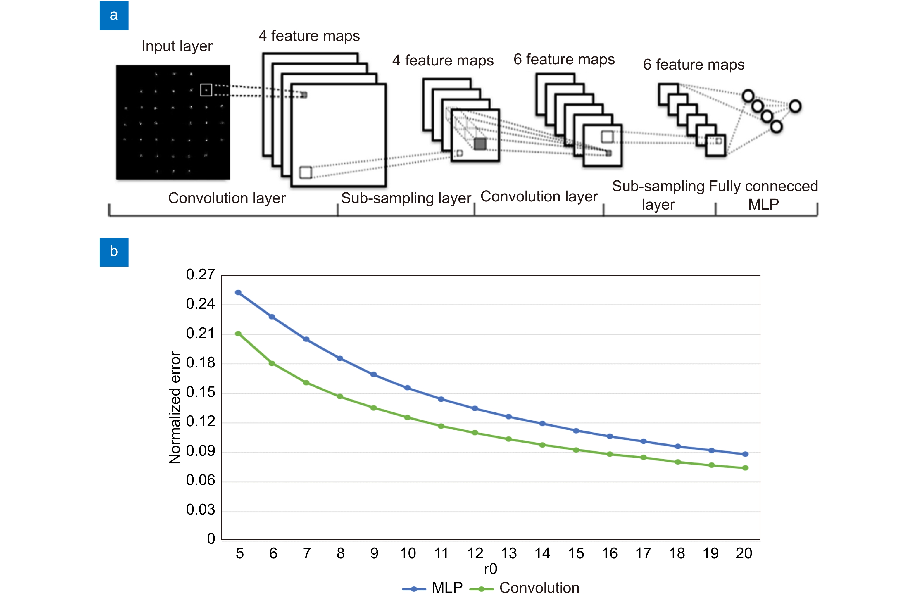
(a) The architecture of the CNN for SHWFS. The input is a SHWFS image and the output is a vector, which indicates centroids. (b) The performance of CNN compared with MLP where the error is calculated as the average of the absolute value of the difference between all the output network centroids and the simulated true centroids. Figure reproduced from: (a, b) ref.74, International Conference on Hybrid Artificial Intelligence Systems.
-
Figure 6.
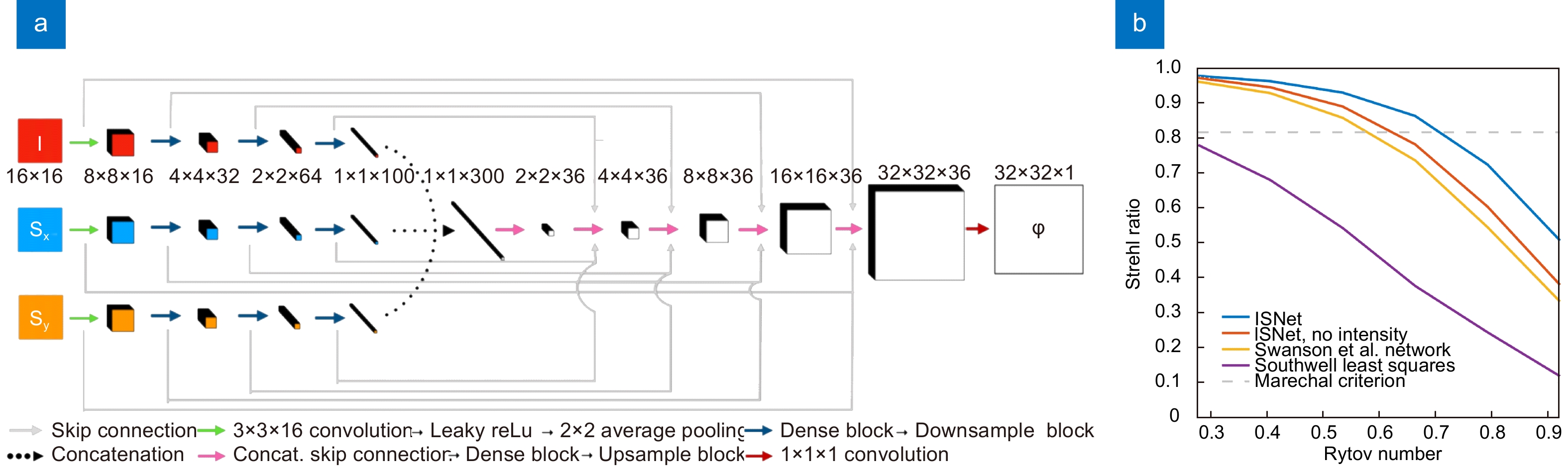
(a) Architecture of ISNet. This network takes three 16×16 inputs (x-slopes, y-slopes and intensities) and outputs a 32×32 unwrapped wavefront. (b) Plot of average Strehl ratio vs. Rytov number for different reconstruction algorithms. For comparison, the Strehl ratio of a Marèchal criterion-limited beam is shown in (b), which is 0.82. Figure reproduced from: (a, b) ref.75, Optical Society of America.
-
Figure 7.
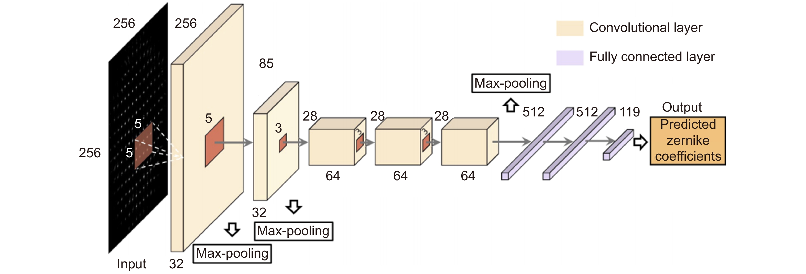
Architecture of LSHWS. The network contains five convolutional layers and three full connected layers. The input is a SHWFS image of size 256×256. The output is a vector of size 119, which represents Zernike coefficients. Figure reproduced from ref.76, Optical Society of America.
-
Figure 8.
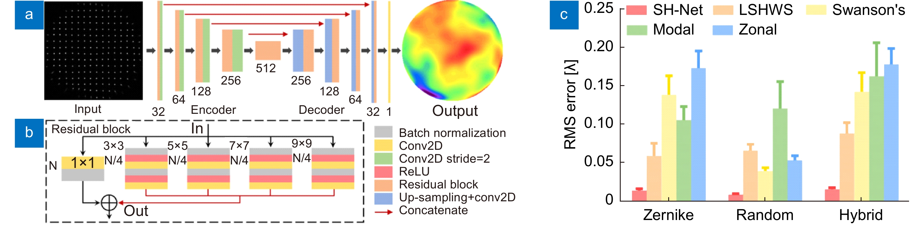
(a) Architecture of SH-Net. The input is a SHWFS image of size 256×256, and the output is a phase map with the same size as the input. (b) the Residual block. ‘N’ and ‘N/4’ indicate the number of channels. (c) Statistical results of RMS wavefront error of five methods in wavefront detection. Figure reproduced from: (a–c) ref.77, Optical Society of America.
-
Figure 9.
Architecture of the deconvolution VGG network (De-VGG). The De-VGG includes convolution layers, batch normalization layer filters, activation function ReLU, and deconvolution layers. The fully connected layers are removed, as the high output order slows down the calculation speed, but the deconvolution layer will not. Figure reproduced from ref.80, under a Creative Commons Attribution License 4.0.
-
Figure 10.
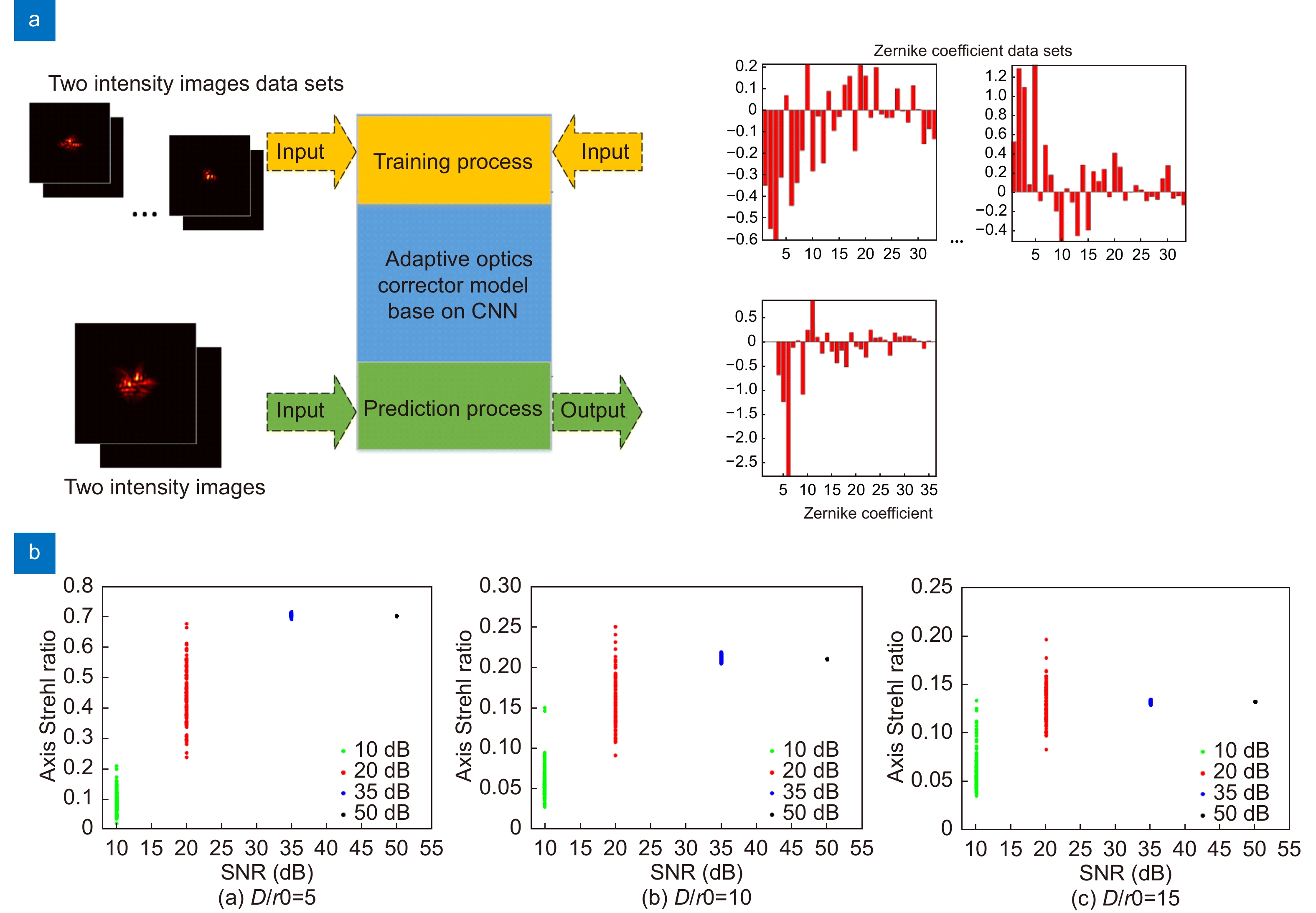
(a) The data flow of the training and inference processes. (b) Strehl ratio of CNN compensation under different SNR conditions. Figure reproduced with permission from: (a, b) ref. 81, Elsevier.
-
Figure 11.
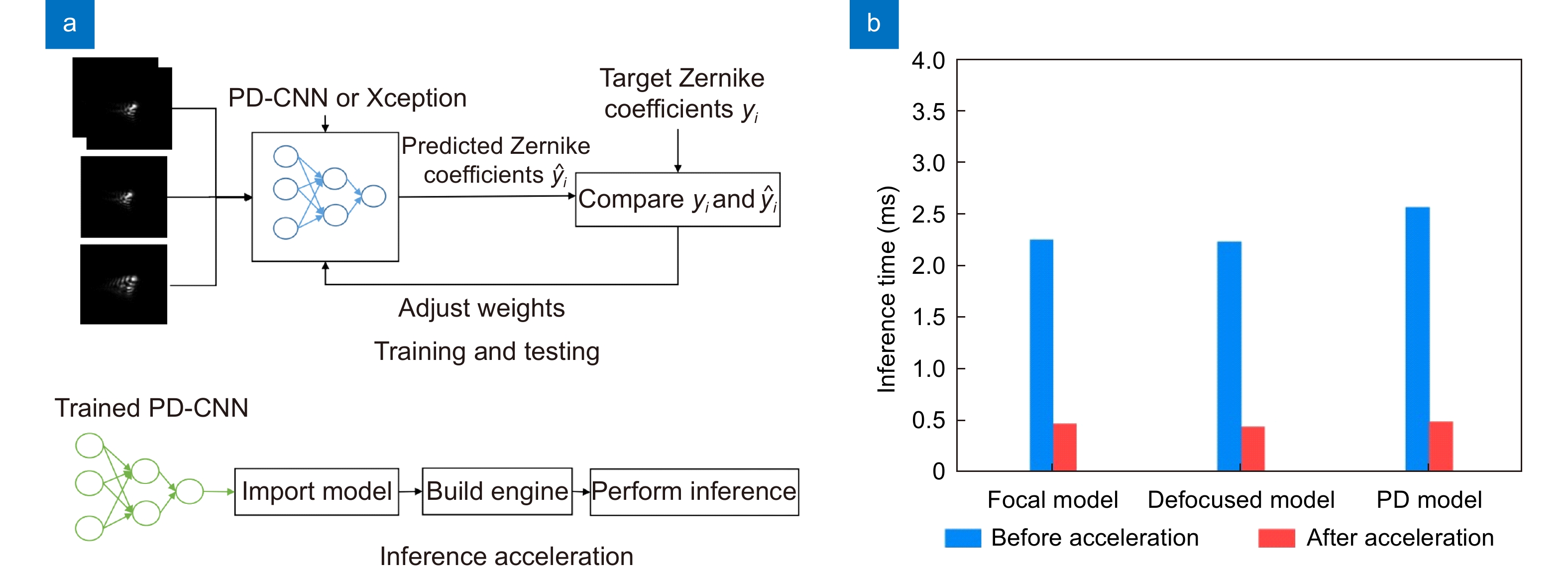
(a) The experiments of training and testing processes and inference acceleration. During training and testing processes, two networks were used, phase-diversity CNN (PD-CNN) and Xception. PD-CNN includes three convolution layers and two full connection layers. For each network, three sets of comparative experiments are set as following, inputting the focal and defocused intensity images separately, and inputting the focal and defocused intensity images at the same time. During the inference acceleration process, the trained model is optimized by TensorRT. (b) The inference time before and after acceleration with NVIDIA GTX 1080Ti. Figure reproduced from: (a, b) ref.82, under a Creative Commons Attribution License 4.0.
-
Figure 12.
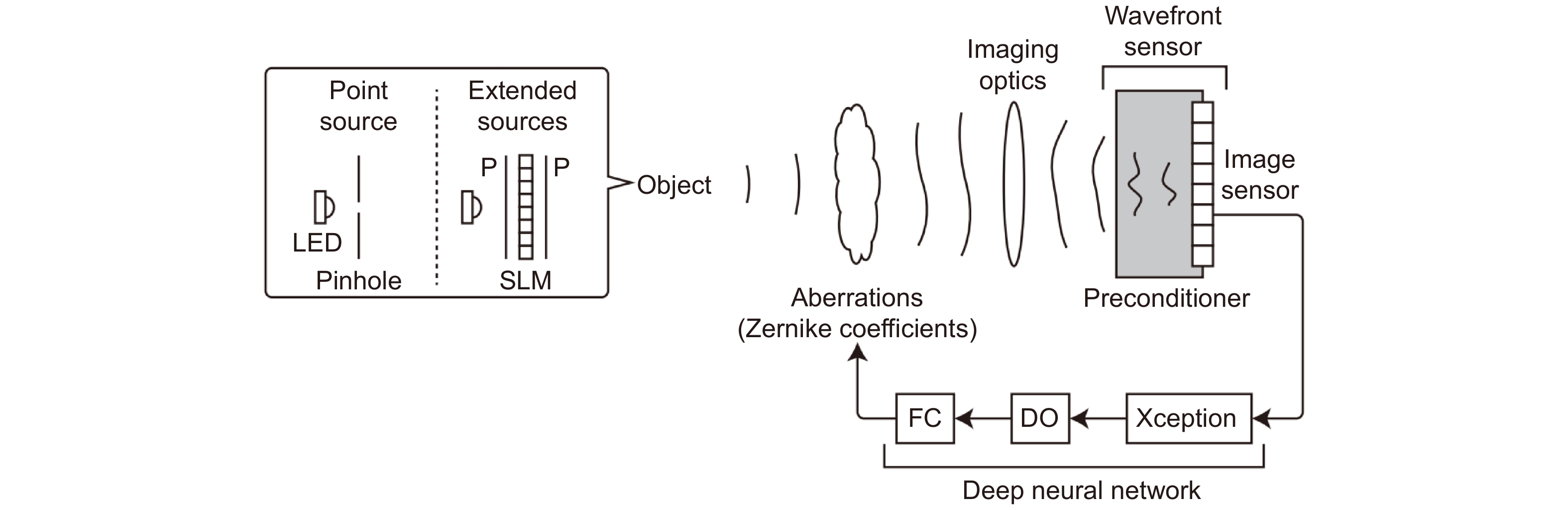
Schematic and experimental diagram of the deep learning wavefront sensor. LED: light emitting diode. P: Polarizer. SLM: Spatial light modulator. DO: Dropout layer. FC: full connection layer. Figure reproduced from ref.83, Optical Society of America.
-
Figure 13.
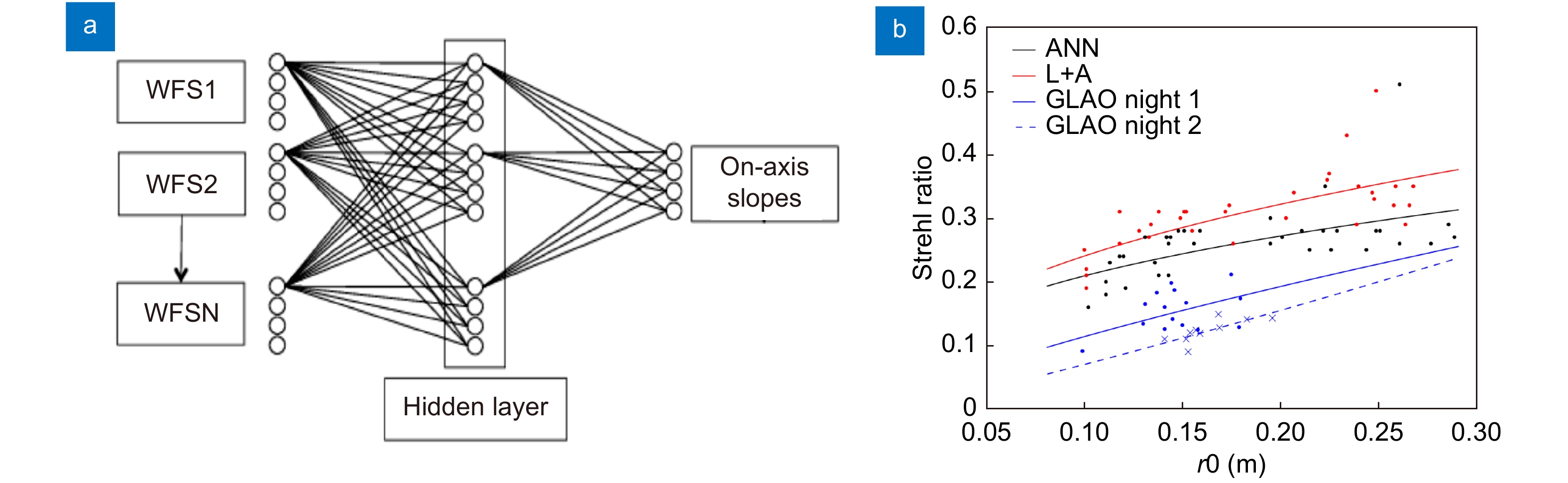
(a) Network diagram for CARMEN. where the inputs are the slopes of off-axis WFSs and the outputs are the on-axis slopes for the target direction. One hidden layer with the same number of neurons as the inputs is used to link the inputs and outputs and the sigmoid activation function is used. (b) On-sky Strehl ratio (in H-band) comparison with different methods. This on-sky experiment was carried out on the 4.2m William-Herschel Telescope. The Strehl ratios achieved by the ANN (CARMEN), the Learn and Apply (L&A) method and two GLAO night performances are compared. Figure reproduced from (a, b) ref.84, Oxford University Press.
-
Figure 14.
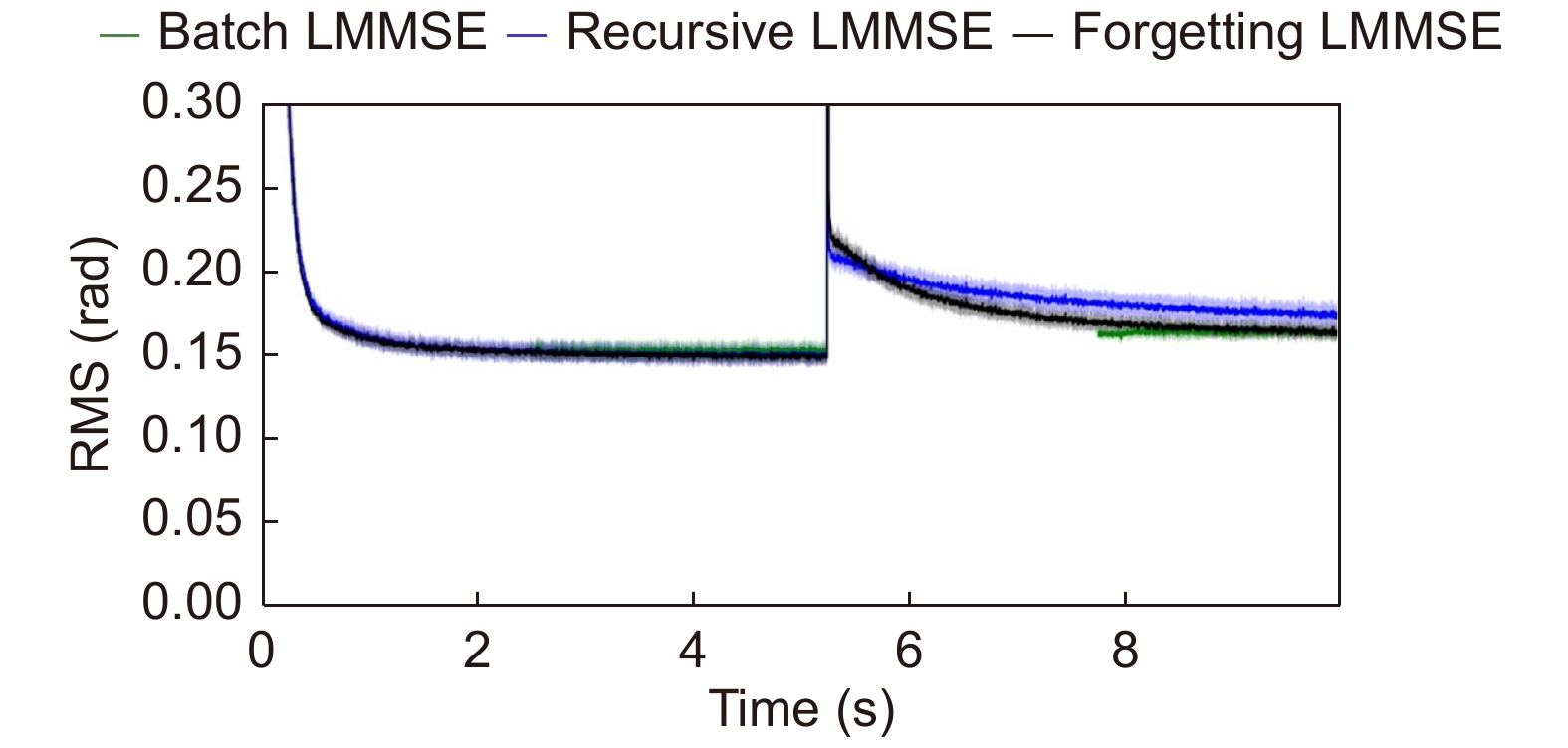
Wind jumps of 7 m/s showing the convergence of the recursive LMMSE (blue) and the forgetting LMMSE (black), as well as the resetting of the batch LMMSE (green) for a regressor with a 3-by-3 spatial grid and five previous measurements for each phase point. Figure reproduced from ref.87, Optical Society of America.
-
Figure 15.
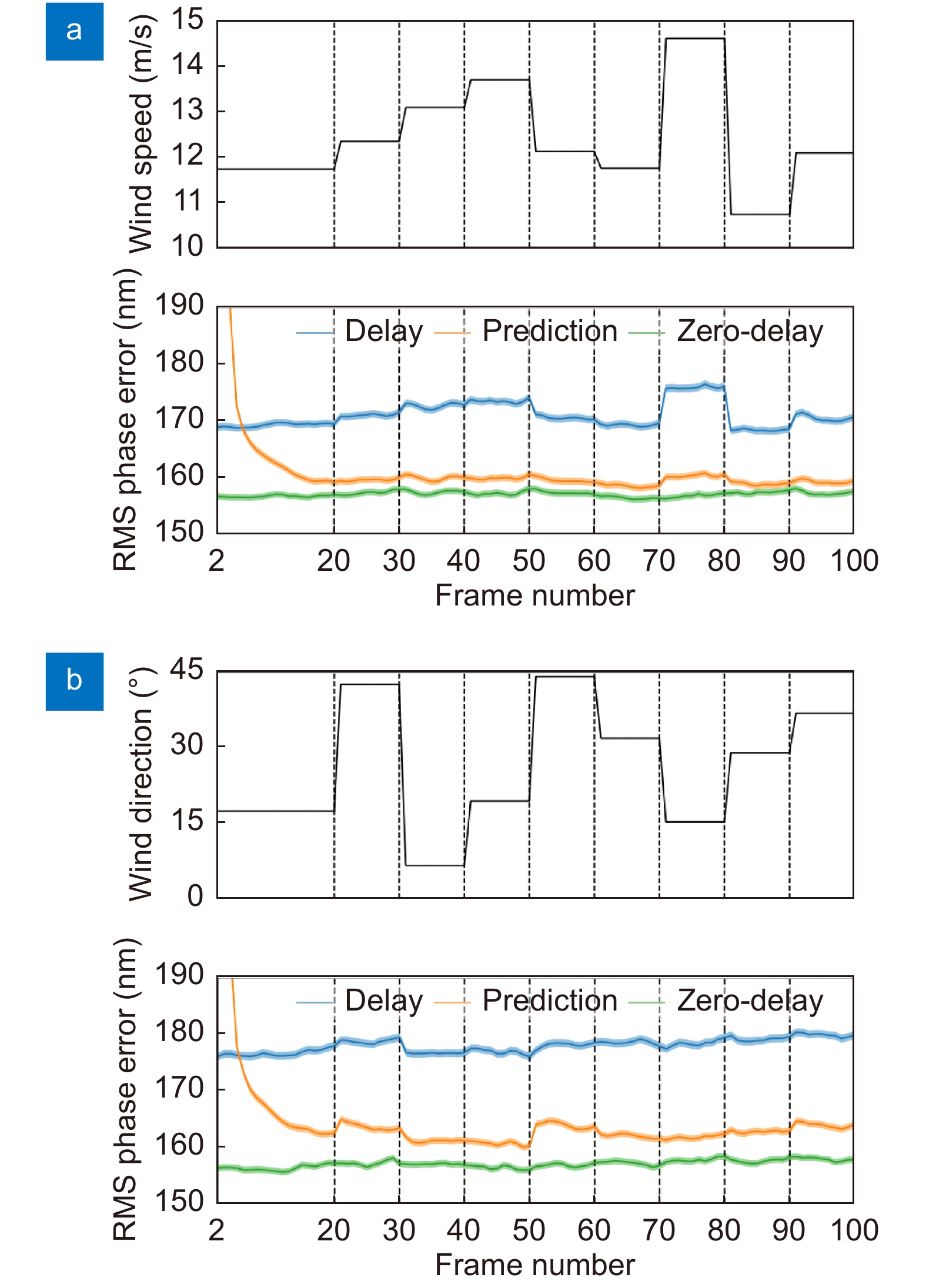
(a) Robustness of the predictor against wind speed fluctuations between 10 and 15 m/s every 10 frames. (b) Robustness of the predictor against wind direction fluctuations between 0 and 45 degrees every 10 frames. Figure reproduced from: (a, b) ref.91, Oxford University Press.
-
Figure 16.
(a) Architecture of the encoder-decoder deconvolution neural network. The details of the architecture are described in Ref.95. (b) Upper panel: end-to-end deconvolution process, where the grey blocks are the deconvolution blocks described in the lower panel. Lower panel: internal architecture of each deconvolution block. Colors for the blocks and the specific details for each block are described in the reference. Figure reproduced from: (a, b) Ref.95, ESO.
-
Figure 17.
Top panels: a single raw image from the burst. Middle panels: reconstructed frames with the recurrent network. Lower panels: azimuthally averaged Fourier power spectra of the images. The left column shows results from the continuum image at 6302 Å while the right column shows the results at the core of the 8542 Å line. All power spectra have been normalized to the value at the largest period. Figure reproduced from ref.95, ESO.
-
Figure 18.
The flowchart of AO image restoration by cGAN. The whole network consists of two parts, generator network and discriminator network, which are used for learning the atmospheric degradation process and achieving the purpose of generating restored images. The loss function of the network is a combination of content loss for generator network and adversarial loss for discriminant network. Figure reproduced from ref.96, SPIE.
-
Figure 19.
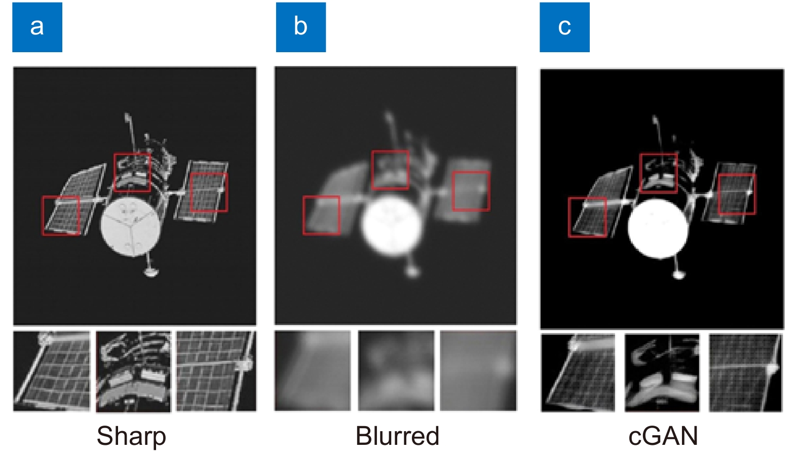
The results of blind restoration for the Hubble telescope. (a) The sharp image, (b) the blurred image by Zernike polynomial method in atmospheric turbulence strength D/r0= 10, and (c) the result of restoration by cGAN, respectively. Figure reproduced from ref.96, SPIE.
-
Figure 20.
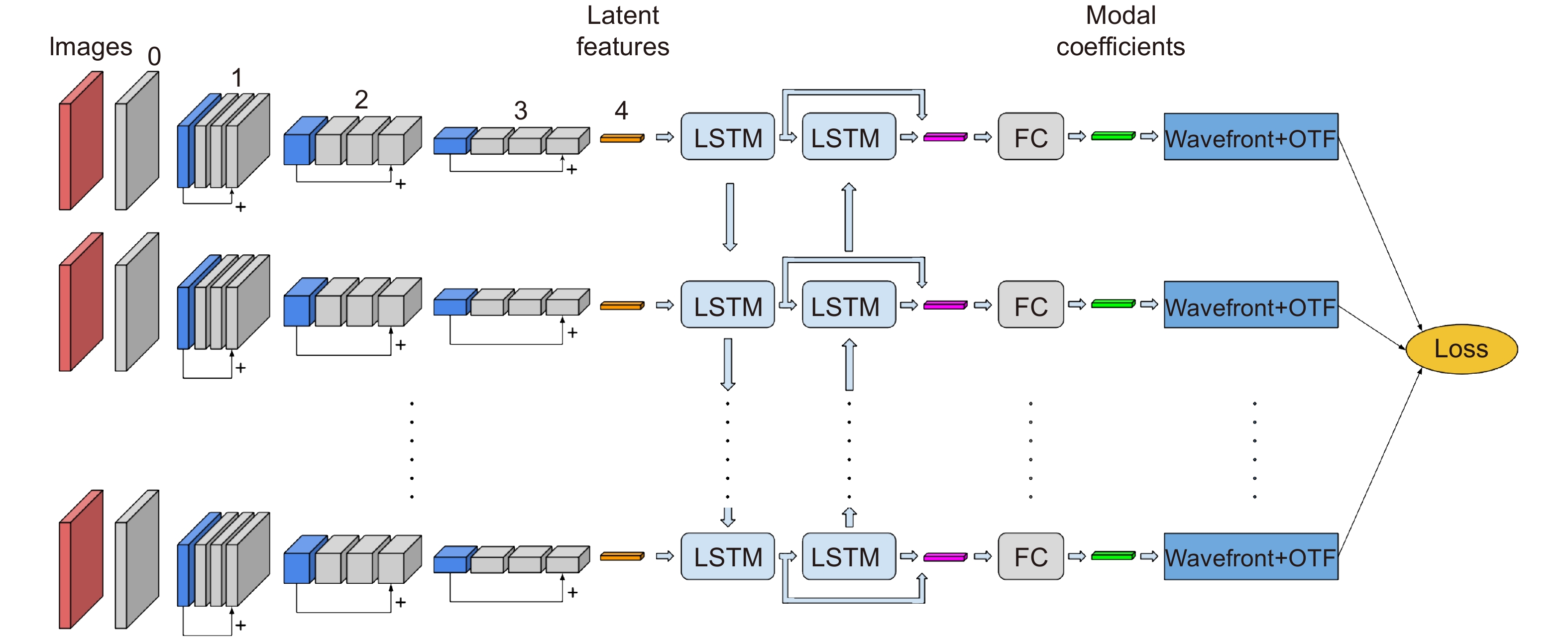
Block diagrams showing the architecture of the network and how it is trained by unsupervised training. Figure reproduced from ref.97, arXiv.
-
Figure 21.
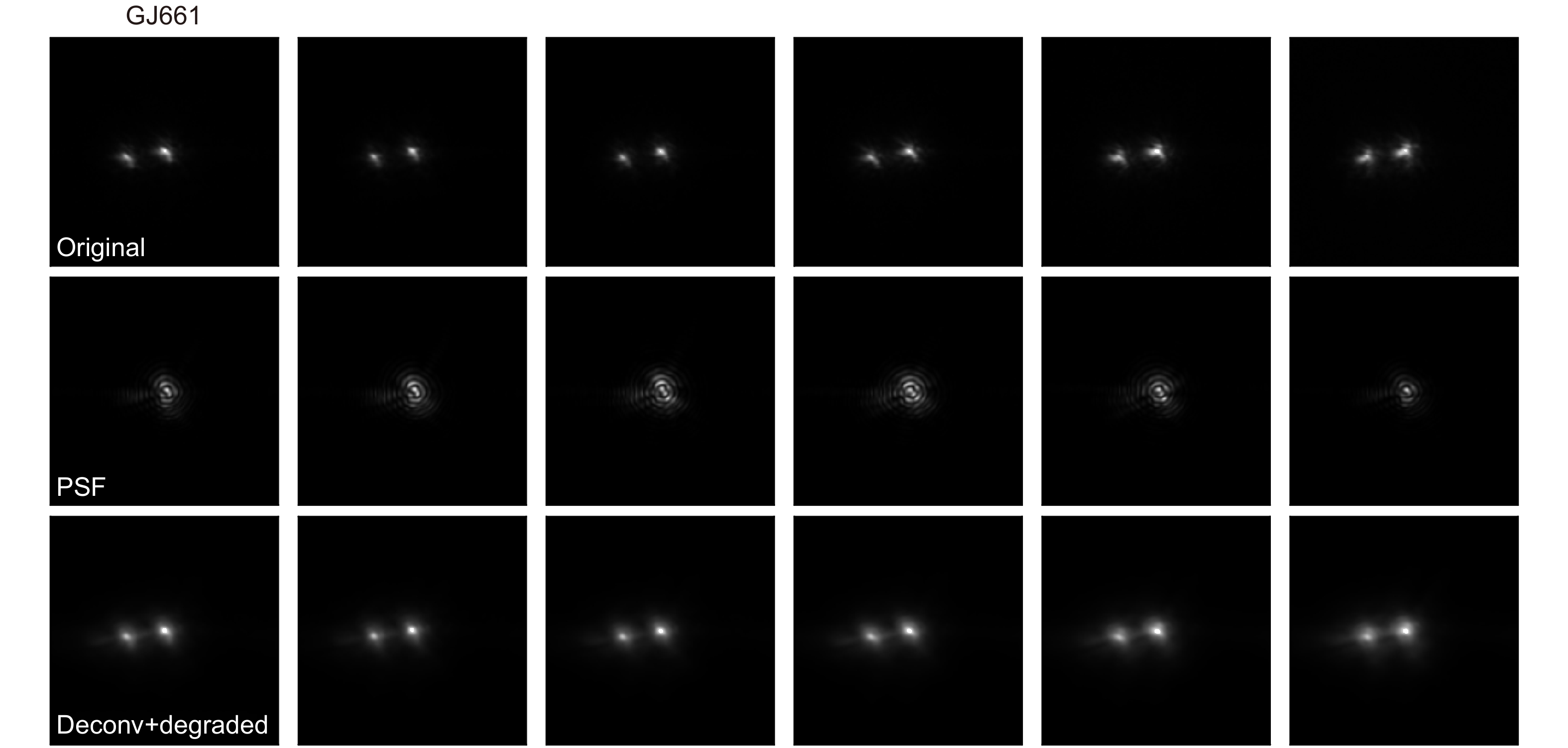
Original frames of the burst (upper row), estimated PSF (middle row) and for the GJ661. The upper row shows six raw frames of the burst. The second row displays the instantaneous PSF estimated by the neural network approach. The last row shows the results from re-convolve the deconvolved image with the estimated PSF. Figure reproduced from ref. 97, arXiv.
-
Figure 22.
Controller for an AOS. (a) PI control model; (b) DLCM control model.
$\text{Z}_{\text{A}}^{-1}$ $\text{Z}_{\text{B}}^{-1}$ $ J $ $ J_{0} $


